Here is the procedure that Breiman is proposing:

1. Randomly choose a subset of the rows of your data (i.e., “bootstrap replicates of your learning set”).
2. Train a model using this subset.
3. Save that model, and then return to step 1 a few times.

This procedure is known as “bagging.” It is based on a deep and important insight: although each of the models trained on a subset of data will make more errors than a model trained on the full dataset, those errors will not be correlated with each other. Different models will make different errors. The average of those errors, therefore, is: zero! So if we take the average of all of the models’ predictions, then we should end up with a prediction that gets closer and closer to the correct answer, the more models we have. This is an extraordinary result—it means that we can improve the accuracy of nearly any kind of machine learning algorithm by training it multiple times, each time on a different random subset of the data, and averaging its predictions.

In 2001 Leo Breiman went on to demonstrate that this approach to building models, when applied to decision tree building algorithms, was particularly powerful. He went even further than just randomly choosing rows for each model’s training, but also randomly selected from a subset of columns when choosing each split in each decision tree. He called this method the random forest. Today it is, perhaps, the most widely used and practically important machine learning method.

In essence a random forest is a model that averages the predictions of a large number of decision trees, which are generated by randomly varying various parameters that specify what data is used to train the tree and other tree parameters. Bagging is a particular approach to “ensembling,” or combining the results of multiple models together. To see how it works in practice, let’s get started on creating our own random forest!

In [43]:

We can create a random forest just like we created a decision tree, except now, we are also specifying parameters that indicate how many trees should be in the forest, how we should subset the data items (the rows), and how we should subset the fields (the columns).

In the following function definition defines the number of trees we want, max_samples defines how many rows to sample for training each tree, and max_features defines how many columns to sample at each split point (where 0.5 means “take half the total number of columns”). We can also specify when to stop splitting the tree nodes, effectively limiting the depth of the tree, by including the same min_samples_leaf parameter we used in the last section. Finally, we pass n_jobs=-1 to tell sklearn to use all our CPUs to build the trees in parallel. By creating a little function for this, we can more quickly try different variations in the rest of this chapter:

In [44]:

def rf(xs, y, n_estimators=40, max_samples=200_000,
       max_features=0.5, min_samples_leaf=5, **kwargs):
    return RandomForestRegressor(n_jobs=-1, n_estimators=n_estimators,
        min_samples_leaf=min_samples_leaf, oob_score=True).fit(xs, y)

In [45]:

In [46]:

Out[46]:

(0.170917, 0.233975)

One of the most important properties of random forests is that they aren’t very sensitive to the hyperparameter choices, such as max_features. You can set n_estimators to as high a number as you have time to train—the more trees you have, the more accurate the model will be. max_samples can often be left at its default, unless you have over 200,000 data points, in which case setting it to 200,000 will make it train faster with little impact on accuracy. max_features=0.5 and both tend to work well, although sklearn’s defaults work well too.

The sklearn docs of the effects of different max_features choices, with increasing numbers of trees. In the plot, the blue plot line uses the fewest features and the green line uses the most (it uses all the features). As you can see in <>, the models with the lowest error result from using a subset of features but with a larger number of trees.

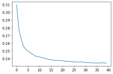
To see the impact of n_estimators, let’s get the predictions from each individual tree in our forest (these are in the estimators_ attribute):

In [47]:

preds = np.stack([t.predict(valid_xs) for t in m.estimators_])

As you can see, preds.mean(0) gives the same results as our random forest:

In [48]:

Out[48]:

0.233975

In [49]:

plt.plot([r_mse(preds[:i+1].mean(0), valid_y) for i in range(40)]);

The performance on our validation set is worse than on our training set. But is that because we’re overfitting, or because the validation set covers a different time period, or a bit of both? With the existing information we’ve seen, we can’t tell. However, random forests have a very clever trick called out-of-bag (OOB) error that can help us with this (and more!).

Out-of-Bag Error

Recall that in a random forest, each tree is trained on a different subset of the training data. The OOB error is a way of measuring prediction error on the training set by only including in the calculation of a row’s error trees where that row was not included in training. This allows us to see whether the model is overfitting, without needing a separate validation set.

A: My intuition for this is that, since every tree was trained with a different randomly selected subset of rows, out-of-bag error is a little like imagining that every tree therefore also has its own validation set. That validation set is simply the rows that were not selected for that tree’s training.

This is particularly beneficial in cases where we have only a small amount of training data, as it allows us to see whether our model generalizes without removing items to create a validation set. The OOB predictions are available in the oob_prediction_ attribute. Note that we compare them to the training labels, since this is being calculated on trees using the training set.

In [50]:

Out[50]:

We can see that our OOB error is much lower than our validation set error. This means that something else is causing that error, in addition to normal generalization error. We’ll discuss the reasons for this later in this chapter.

This is one way to interpret our model’s predictions—let’s focus on more of those now.