Instead, it would be best to learn the values of the kernels. We already know how to do this—SGD! In effect, the model will learn the features that are useful for classification.

When we use convolutions instead of (or in addition to) regular linear layers we create a convolutional neural network (CNN).

Let’s go back to the basic neural network we had in <>. It was defined like this:

In [ ]:

We can view a model’s definition:

In [ ]:

Out[ ]:

Sequential(
  (0): Linear(in_features=784, out_features=30, bias=True)
  (1): ReLU()
  (2): Linear(in_features=30, out_features=1, bias=True)
)

We now want to create a similar architecture to this linear model, but using convolutional layers instead of linear. nn.Conv2d is the module equivalent of F.conv2d. It’s more convenient than F.conv2d when creating an architecture, because it creates the weight matrix for us automatically when we instantiate it.

Here’s a possible architecture:

In [ ]:

broken_cnn = sequential(
    nn.Conv2d(1,30, kernel_size=3, padding=1),
    nn.Conv2d(30,1, kernel_size=3, padding=1)
)

One thing to note here is that we didn’t need to specify 28×28 as the input size. That’s because a linear layer needs a weight in the weight matrix for every pixel, so it needs to know how many pixels there are, but a convolution is applied over each pixel automatically. The weights only depend on the number of input and output channels and the kernel size, as we saw in the previous section.

Think about what the output shape is going to be, then let’s try it and see:

In [ ]:

broken_cnn(xb).shape

Out[ ]:

torch.Size([64, 1, 28, 28])

This is not something we can use to do classification, since we need a single output activation per image, not a 28×28 map of activations. One way to deal with this is to use enough stride-2 convolutions such that the final layer is size 1. That is, after one stride-2 convolution the size will be 14×14, after two it will be 7×7, then 4×4, 2×2, and finally size 1.

Let’s try that now. First, we’ll define a function with the basic parameters we’ll use in each convolution:

In [ ]:

When we use a stride-2 convolution, we often increase the number of features at the same time. This is because we’re decreasing the number of activations in the activation map by a factor of 4; we don’t want to decrease the capacity of a layer by too much at a time.

Here is how we can build a simple CNN:

In [ ]:

simple_cnn = sequential(
    conv(1 ,4),            #14x14
    conv(4 ,8),            #7x7
    conv(8 ,16),           #4x4
    conv(32,2, act=False), #1x1
    Flatten(),
)

Now the network outputs two activations, which map to the two possible levels in our labels:

In [ ]:

Out[ ]:

torch.Size([64, 2])

We can now create our Learner:

In [ ]:

learn = Learner(dls, simple_cnn, loss_func=F.cross_entropy, metrics=accuracy)

To see exactly what’s going on in the model, we can use summary:

In [ ]:

learn.summary()

Out[ ]:

Note that the output of the final Conv2d layer is 64x2x1x1. We need to remove those extra 1x1 axes; that’s what Flatten does. It’s basically the same as PyTorch’s squeeze method, but as a module.

Let’s see if this trains! Since this is a deeper network than we’ve built from scratch before, we’ll use a lower learning rate and more epochs:

In [ ]:

learn.fit_one_cycle(2, 0.01)

Success! It’s getting closer to the resnet18 result we had, although it’s not quite there yet, and it’s taking more epochs, and we’re needing to use a lower learning rate. We still have a few more tricks to learn, but we’re getting closer and closer to being able to create a modern CNN from scratch.

We can see from the summary that we have an input of size 64x1x28x28. The axes are batch,channel,height,width. This is often represented as NCHW (where refers to batch size). Tensorflow, on the other hand, uses NHWC axis order. The first layer is:

In [ ]:

m = learn.model[0]
m

Out[ ]:

Sequential(
  (0): Conv2d(1, 4, kernel_size=(3, 3), stride=(2, 2), padding=(1, 1))
  (1): ReLU()
)

So we have 1 input channel, 4 output channels, and a 3×3 kernel. Let’s check the weights of the first convolution:

In [ ]:

m[0].weight.shape

Out[ ]:

torch.Size([4, 1, 3, 3])

The summary shows we have 40 parameters, and 4*1*3*3 is 36. What are the other four parameters? Let’s see what the bias contains:

In [ ]:

Out[ ]:

We can now use this information to clarify our statement in the previous section: “When we use a stride-2 convolution, we often increase the number of features because we’re decreasing the number of activations in the activation map by a factor of 4; we don’t want to decrease the capacity of a layer by too much at a time.”

What happened here is that our stride-2 convolution halved the grid size from 14x14 to 7x7, and we doubled the number of filters from 8 to 16, resulting in no overall change in the amount of computation. If we left the number of channels the same in each stride-2 layer, the amount of computation being done in the net would get less and less as it gets deeper. But we know that the deeper layers have to compute semantically rich features (such as eyes or fur), so we wouldn’t expect that doing less computation would make sense.

Another way to think of this is based on receptive fields.

The receptive field is the area of an image that is involved in the calculation of a layer. On the , you’ll find an Excel spreadsheet called conv-example.xlsx that shows the calculation of two stride-2 convolutional layers using an MNIST digit. Each layer has a single kernel. <> shows what we see if we click on one of the cells in the conv2 section, which shows the output of the second convolutional layer, and click trace precedents.

Here, the cell with the green border is the cell we clicked on, and the blue highlighted cells are its precedents—that is, the cells used to calculate its value. These cells are the corresponding 3×3 area of cells from the input layer (on the left), and the cells from the filter (on the right). Let’s now click trace precedents again, to see what cells are used to calculate these inputs. <> shows what happens.

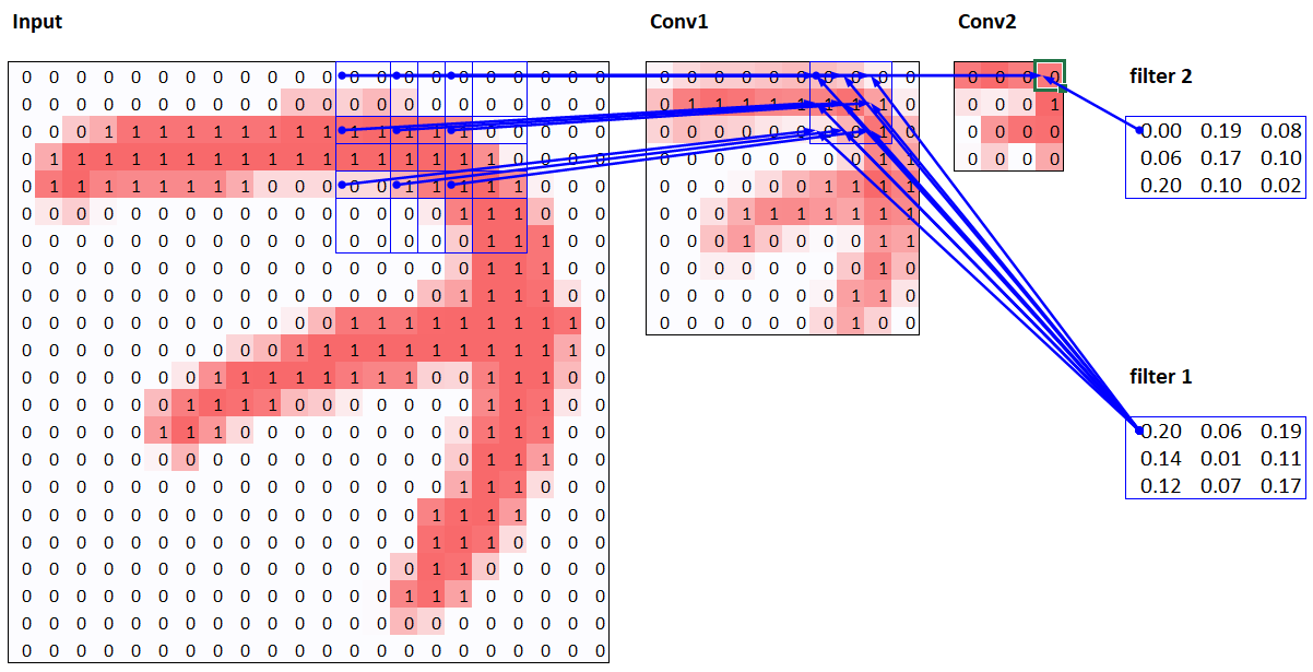
In this example, we have just two convolutional layers, each of stride 2, so this is now tracing right back to the input image. We can see that a 7×7 area of cells in the input layer is used to calculate the single green cell in the Conv2 layer. This 7×7 area is the receptive field in the input of the green activation in Conv2. We can also see that a second filter kernel is needed now, since we have two layers.

As you see from this example, the deeper we are in the network (specifically, the more stride-2 convs we have before a layer), the larger the receptive field for an activation in that layer. A large receptive field means that a large amount of the input image is used to calculate each activation in that layer is. We now know that in the deeper layers of the network we have semantically rich features, corresponding to larger receptive fields. Therefore, we’d expect that we’d need more weights for each of our features to handle this increasing complexity. This is another way of saying the same thing we mentioned in the previous section: when we introduce a stride-2 conv in our network, we should also increase the number of channels.

When writing this particular chapter, we had a lot of questions we needed answers for, to be able to explain CNNs to you as best we could. Believe it or not, we found most of the answers on Twitter. We’re going to take a quick break to talk to you about that now, before we move on to color images.

We are not, to say the least, big users of social networks in general. But our goal in writing this book is to help you become the best deep learning practitioner you can, and we would be remiss not to mention how important Twitter has been in our own deep learning journeys.

You see, there’s another part of Twitter, far away from Donald Trump and the Kardashians, which is the part of Twitter where deep learning researchers and practitioners talk shop every day. As we were writing this section, Jeremy wanted to double-check that what we were saying about stride-2 convolutions was accurate, so he asked on Twitter:

A few minutes later, this answer popped up:

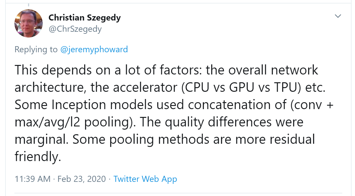
Christian Szegedy is the first author of Inception, the 2014 ImageNet winner and source of many key insights used in modern neural networks. Two hours later, this appeared:

Do you recognize that name? You saw it in <>, when we were talking about the Turing Award winners who established the foundations of deep learning today!

Jeremy also asked on Twitter for help checking our description of label smoothing in <> was accurate, and got a response again from directly from Christian Szegedy (label smoothing was originally introduced in the Inception paper):

Many of the top people in deep learning today are Twitter regulars, and are very open about interacting with the wider community. One good way to get started is to look at a list of Jeremy’s , or Sylvain’s. That way, you can see a list of Twitter users that we think have interesting and useful things to say.

Twitter is the main way we both stay up to date with interesting papers, software releases, and other deep learning news. For making connections with the deep learning community, we recommend getting involved both in the and on Twitter.

That said, let’s get back to the meat of this chapter. Up until now, we have only shown you examples of pictures in black and white, with one value per pixel. In practice, most colored images have three values per pixel to define their color. We’ll look at working with color images next.