
We don’t have a lot of data for our problem (150 pictures of each sort of bear at most), so to train our model, we’ll use with an image size of 224 px, which is fairly standard for image classification, and default aug_transforms:
In [ ]:
We can now create our Learner and fine-tune it in the usual way:
In [ ]:
learn = cnn_learner(dls, resnet18, metrics=error_rate)
| epoch | train_loss | valid_loss | error_rate | time |
|---|---|---|---|---|
| 0 | 0.213371 | 0.112450 | 0.023810 | 00:05 |
| 1 | 0.173855 | 0.072306 | 0.023810 | 00:06 |
| 2 | 0.147096 | 0.039068 | 0.015873 | 00:06 |
| 3 | 0.123984 | 0.026801 | 0.015873 | 00:06 |
Now let’s see whether the mistakes the model is making are mainly thinking that grizzlies are teddies (that would be bad for safety!), or that grizzlies are black bears, or something else. To visualize this, we can create a confusion matrix:
In [ ]:
It’s helpful to see where exactly our errors are occurring, to see whether they’re due to a dataset problem (e.g., images that aren’t bears at all, or are labeled incorrectly, etc.), or a model problem (perhaps it isn’t handling images taken with unusual lighting, or from a different angle, etc.). To do this, we can sort our images by their loss.
The loss is a number that is higher if the model is incorrect (especially if it’s also confident of its incorrect answer), or if it’s correct, but not confident of its correct answer. In a couple of chapters we’ll learn in depth how loss is calculated and used in the training process. For now, shows us the images with the highest loss in our dataset. As the title of the output says, each image is labeled with four things: prediction, actual (target label), loss, and probability. The probability here is the confidence level, from zero to one, that the model has assigned to its prediction:
In [ ]:
interp.plot_top_losses(5, nrows=1)
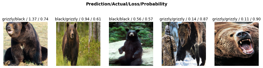
This output shows that the image with the highest loss is one that has been predicted as “grizzly” with high confidence. However, it’s labeled (based on our Bing image search) as “black.” We’re not bear experts, but it sure looks to us like this label is incorrect! We should probably change its label to “grizzly.”
The intuitive approach to doing data cleaning is to do it before you train a model. But as you’ve seen in this case, a model can actually help you find data issues more quickly and easily. So, we normally prefer to train a quick and simple model first, and then use it to help us with data cleaning.
fastai includes a handy GUI for data cleaning called ImageClassifierCleaner that allows you to choose a category and the training versus validation set and view the highest-loss images (in order), along with menus to allow images to be selected for removal or relabeling:
In [ ]:
# for idx in cleaner.delete(): cleaner.fns[idx].unlink()
We can see that amongst our “black bears” is an image that contains two bears: one grizzly, one black. So, we should choose <Delete> in the menu under this image. ImageClassifierCleaner doesn’t actually do the deleting or changing of labels for you; it just returns the indices of items to change. So, for instance, to delete (unlink) all images selected for deletion, we would run:
To move images for which we’ve selected a different category, we would run:
for idx,cat in cleaner.change(): shutil.move(str(cleaner.fns[idx]), path/cat)
We’ll be seeing more examples of model-driven data cleaning throughout this book. Once we’ve cleaned up our data, we can retrain our model. Try it yourself, and see if your accuracy improves!
note: No Need for Big Data: After cleaning the dataset using these steps, we generally are seeing 100% accuracy on this task. We even see that result when we download a lot fewer images than the 150 per class we’re using here. As you can see, the common complaint that you need massive amounts of data to do deep learning can be a very long way from the truth!

