Let’s grab the data—we’ll use the already-resized 160 px version to make things faster still, and will random crop to 128 px:

In [ ]:

In [ ]:

In [ ]:

dls.show_batch(max_n=4)

When we looked at MNIST we were dealing with 28×28-pixel images. For Imagenette we are going to be training with 128×128-pixel images. Later, we would like to be able to use larger images as well—at least as big as 224×224 pixels, the ImageNet standard. Do you recall how we managed to get a single vector of activations for each image out of the MNIST convolutional neural network?

The approach we used was to ensure that there were enough stride-2 convolutions such that the final layer would have a grid size of 1. Then we just flattened out the unit axes that we ended up with, to get a vector for each image (so, a matrix of activations for a mini-batch). We could do the same thing for Imagenette, but that would cause two problems:

• We’d need lots of stride-2 layers to make our grid 1×1 at the end—perhaps more than we would otherwise choose.
• The model would not work on images of any size other than the size we originally trained on.

This problem was solved through the creation of fully convolutional networks. The trick in fully convolutional networks is to take the average of activations across a convolutional grid. In other words, we can simply use this function:

In [ ]:

As you see, it is taking the mean over the x- and y-axes. This function will always convert a grid of activations into a single activation per image. PyTorch provides a slightly more versatile module called nn.AdaptiveAvgPool2d, which averages a grid of activations into whatever sized destination you require (although we nearly always use a size of 1).

A fully convolutional network, therefore, has a number of convolutional layers, some of which will be stride 2, at the end of which is an adaptive average pooling layer, a flatten layer to remove the unit axes, and finally a linear layer. Here is our first fully convolutional network:

In [ ]:

def block(ni, nf): return ConvLayer(ni, nf, stride=2)
def get_model():
        block(3, 16),
        block(16, 32),
        block(32, 64),
        block(128, 256),
        nn.AdaptiveAvgPool2d(1),
        nn.Linear(256, dls.c))

We’re going to be replacing the implementation of block in the network with other variants in a moment, which is why we’re not calling it conv any more. We’re also saving some time by taking advantage of fastai’s ConvLayer, which that already provides the functionality of conv from the last chapter (plus a lot more!).

This is different from regular pooling in the sense that those layers will generally take the average (for average pooling) or the maximum (for max pooling) of a window of a given size. For instance, max pooling layers of size 2, which were very popular in older CNNs, reduce the size of our image by half on each dimension by taking the maximum of each 2×2 window (with a stride of 2).

As before, we can define a Learner with our custom model and then train it on the data we grabbed earlier:

In [ ]:

def get_learner(m):
    return Learner(dls, m, loss_func=nn.CrossEntropyLoss(), metrics=accuracy
                  ).to_fp16()
learn = get_learner(get_model())

In [ ]:

Out[ ]:

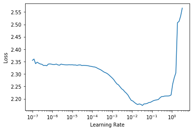
3e-3 is often a good learning rate for CNNs, and that appears to be the case here too, so let’s try that:

That’s a pretty good start, considering we have to pick the correct one of 10 categories, and we’re training from scratch for just 5 epochs! We can do way better than this using a deeper mode, but just stacking new layers won’t really improve our results (you can try and see for yourself!). To work around this problem, ResNets introduce the idea of skip connections. We’ll explore those and other aspects of ResNets in the next section.