
The first thing we need to set when training a model is the learning rate. We saw in the previous chapter that it needs to be just right to train as efficiently as possible, so how do we pick a good one? fastai provides a tool for this.
One of the most important things we can do when training a model is to make sure that we have the right learning rate. If our learning rate is too low, it can take many, many epochs to train our model. Not only does this waste time, but it also means that we may have problems with overfitting, because every time we do a complete pass through the data, we give our model a chance to memorize it.
So let’s just make our learning rate really high, right? Sure, let’s try that and see what happens:
In [ ]:
| epoch | train_loss | valid_loss | error_rate | time |
|---|---|---|---|---|
| 0 | 4.354680 | 3.003533 | 0.834235 | 00:24 |
That doesn’t look good. Here’s what happened. The optimizer stepped in the correct direction, but it stepped so far that it totally overshot the minimum loss. Repeating that multiple times makes it get further and further away, not closer and closer!
What do we do to find the perfect learning rate—not too high, and not too low? In 2015 the researcher Leslie Smith came up with a brilliant idea, called the learning rate finder. His idea was to start with a very, very small learning rate, something so small that we would never expect it to be too big to handle. We use that for one mini-batch, find what the losses are afterwards, and then increase the learning rate by some percentage (e.g., doubling it each time). Then we do another mini-batch, track the loss, and double the learning rate again. We keep doing this until the loss gets worse, instead of better. This is the point where we know we have gone too far. We then select a learning rate a bit lower than this point. Our advice is to pick either:
- One order of magnitude less than where the minimum loss was achieved (i.e., the minimum divided by 10)
- The last point where the loss was clearly decreasing
The learning rate finder computes those points on the curve to help you. Both these rules usually give around the same value. In the first chapter, we didn’t specify a learning rate, using the default value from the fastai library (which is 1e-3):
In [ ]:
In [ ]:
print(f"Minimum/10: {lr_min:.2e}, steepest point: {lr_steep:.2e}")
Minimum/10: 1.00e-02, steepest point: 5.25e-03
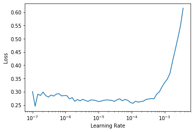
We can see on this plot that in the range 1e-6 to 1e-3, nothing really happens and the model doesn’t train. Then the loss starts to decrease until it reaches a minimum, and then increases again. We don’t want a learning rate greater than 1e-1 as it will give a training that diverges like the one before (you can try for yourself), but 1e-1 is already too high: at this stage we’ve left the period where the loss was decreasing steadily.
In this learning rate plot it appears that a learning rate around 3e-3 would be appropriate, so let’s choose that:
In [ ]:
learn = cnn_learner(dls, resnet34, metrics=error_rate)learn.fine_tune(2, base_lr=3e-3)
| epoch | train_loss | valid_loss | error_rate | time |
|---|---|---|---|---|
| 0 | 1.328591 | 0.344678 | 0.114344 | 00:20 |
It’s interesting that the learning rate finder was only discovered in 2015, while neural networks have been under development since the 1950s. Throughout that time finding a good learning rate has been, perhaps, the most important and challenging issue for practitioners. The solution does not require any advanced maths, giant computing resources, huge datasets, or anything else that would make it inaccessible to any curious researcher. Furthermore, Leslie Smith, was not part of some exclusive Silicon Valley lab, but was working as a naval researcher. All of this is to say: breakthrough work in deep learning absolutely does not require access to vast resources, elite teams, or advanced mathematical ideas. There is lots of work still to be done that requires just a bit of common sense, creativity, and tenacity.
Now that we have a good learning rate to train our model, let’s look at how we can fine-tune the weights of a pretrained model.
We discussed briefly in <> how transfer learning works. We saw that the basic idea is that a pretrained model, trained potentially on millions of data points (such as ImageNet), is fine-tuned for some other task. But what does this really mean?
We now know that a convolutional neural network consists of many linear layers with a nonlinear activation function between each pair, followed by one or more final linear layers with an activation function such as softmax at the very end. The final linear layer uses a matrix with enough columns such that the output size is the same as the number of classes in our model (assuming that we are doing classification).
This final linear layer is unlikely to be of any use for us when we are fine-tuning in a transfer learning setting, because it is specifically designed to classify the categories in the original pretraining dataset. So when we do transfer learning we remove it, throw it away, and replace it with a new linear layer with the correct number of outputs for our desired task (in this case, there would be 37 activations).
This newly added linear layer will have entirely random weights. Therefore, our model prior to fine-tuning has entirely random outputs. But that does not mean that it is an entirely random model! All of the layers prior to the last one have been carefully trained to be good at image classification tasks in general. As we saw in the images from the in <> (see <> through <>), the first few layers encode very general concepts, such as finding gradients and edges, and later layers encode concepts that are still very useful for us, such as finding eyeballs and fur.
Our challenge when fine-tuning is to replace the random weights in our added linear layers with weights that correctly achieve our desired task (classifying pet breeds) without breaking the carefully pretrained weights and the other layers. There is actually a very simple trick to allow this to happen: tell the optimizer to only update the weights in those randomly added final layers. Don’t change the weights in the rest of the neural network at all. This is called freezing those pretrained layers.
When we create a model from a pretrained network fastai automatically freezes all of the pretrained layers for us. When we call the fine_tune method fastai does two things:
- Trains the randomly added layers for one epoch, with all other layers frozen
- Unfreezes all of the layers, and trains them all for the number of epochs requested
Although this is a reasonable default approach, it is likely that for your particular dataset you may get better results by doing things slightly differently. The fine_tune method has a number of parameters you can use to change its behavior, but it might be easiest for you to just call the underlying methods directly if you want to get some custom behavior. Remember that you can see the source code for the method by using the following syntax:
So let’s try doing this manually ourselves. First of all we will train the randomly added layers for three epochs, using fit_one_cycle. As mentioned in <>, fit_one_cycle is the suggested way to train models without using . We’ll see why later in the book; in short, what fit_one_cycle does is to start training at a low learning rate, gradually increase it for the first section of training, and then gradually decrease it again for the last section of training.
In [ ]:
learn.fine_tune??
In [ ]:
learn = cnn_learner(dls, resnet34, metrics=error_rate)
| epoch | train_loss | valid_loss | error_rate | time |
|---|---|---|---|---|
| 0 | 1.188042 | 0.355024 | 0.102842 | 00:20 |
| 1 | 0.534234 | 0.302453 | 0.094723 | 00:20 |
| 2 | 0.325031 | 0.222268 | 0.074425 | 00:20 |
Then we’ll unfreeze the model:
In [ ]:
learn.unfreeze()
and run lr_find again, because having more layers to train, and weights that have already been trained for three epochs, means our previously found learning rate isn’t appropriate any more:
In [ ]:
learn.lr_find()
Out[ ]:
Note that the graph is a little different from when we had random weights: we don’t have that sharp descent that indicates the model is training. That’s because our model has been trained already. Here we have a somewhat flat area before a sharp increase, and we should take a point well before that sharp increase—for instance, 1e-5. The point with the maximum gradient isn’t what we look for here and should be ignored.
Let’s train at a suitable learning rate:
In [ ]:
learn.fit_one_cycle(6, lr_max=1e-5)
| epoch | train_loss | valid_loss | error_rate | time |
|---|---|---|---|---|
| 0 | 0.263579 | 0.217419 | 0.069012 | 00:24 |
| 1 | 0.253060 | 0.210346 | 0.062923 | 00:24 |
| 2 | 0.224340 | 0.207357 | 0.060217 | 00:24 |
| 3 | 0.200195 | 0.207244 | 0.061570 | 00:24 |
| 4 | 0.194269 | 0.200149 | 0.059540 | 00:25 |
| 5 | 0.173164 | 0.202301 | 0.059540 | 00:25 |
This has improved our model a bit, but there’s more we can do. The deepest layers of our pretrained model might not need as high a learning rate as the last ones, so we should probably use different learning rates for those—this is known as using discriminative learning rates.
Even after we unfreeze, we still care a lot about the quality of those pretrained weights. We would not expect that the best learning rate for those pretrained parameters would be as high as for the randomly added parameters, even after we have tuned those randomly added parameters for a few epochs. Remember, the pretrained weights have been trained for hundreds of epochs, on millions of images.
In addition, do you remember the images we saw in <>, showing what each layer learns? The first layer learns very simple foundations, like edge and gradient detectors; these are likely to be just as useful for nearly any task. The later layers learn much more complex concepts, like “eye” and “sunset,” which might not be useful in your task at all (maybe you’re classifying car models, for instance). So it makes sense to let the later layers fine-tune more quickly than earlier layers.
Therefore, fastai’s default approach is to use discriminative learning rates. This was originally developed in the ULMFiT approach to NLP transfer learning that we will introduce in <>. Like many good ideas in deep learning, it is extremely simple: use a lower learning rate for the early layers of the neural network, and a higher learning rate for the later layers (and especially the randomly added layers). The idea is based on insights developed by Jason Yosinski, who showed in 2014 that with transfer learning different layers of a neural network should train at different speeds, as seen in <>.
In [ ]:
learn.fit_one_cycle(3, 3e-3)learn.unfreeze()learn.fit_one_cycle(12, lr_max=slice(1e-6,1e-4))
| epoch | train_loss | valid_loss | error_rate | time |
|---|---|---|---|---|
| 0 | 0.257977 | 0.205400 | 0.067659 | 00:25 |
| 1 | 0.246763 | 0.205107 | 0.066306 | 00:25 |
| 2 | 0.240595 | 0.193848 | 0.062246 | 00:25 |
| 3 | 0.209988 | 0.198061 | 0.062923 | 00:25 |
| 4 | 0.194756 | 0.193130 | 0.064276 | 00:25 |
| 5 | 0.169985 | 0.187885 | 0.056157 | 00:25 |
| 6 | 0.153205 | 0.186145 | 0.058863 | 00:25 |
| 7 | 0.141480 | 0.185316 | 0.053451 | 00:25 |
| 8 | 0.128564 | 0.180999 | 0.051421 | 00:25 |
| 9 | 0.126941 | 0.186288 | 0.054127 | 00:25 |
| 10 | 0.130064 | 0.181764 | 0.054127 | 00:25 |
| 11 | 0.124281 | 0.181855 | 0.054127 | 00:25 |
Now the fine-tuning is working great!
fastai can show us a graph of the training and validation loss:
In [ ]:
learn.recorder.plot_loss()
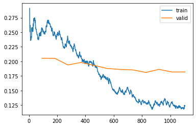
As you can see, the training loss keeps getting better and better. But notice that eventually the validation loss improvement slows, and sometimes even gets worse! This is the point at which the model is starting to over fit. In particular, the model is becoming overconfident of its predictions. But this does not mean that it is getting less accurate, necessarily. Take a look at the table of training results per epoch, and you will often see that the accuracy continues improving, even as the validation loss gets worse. In the end what matters is your accuracy, or more generally your chosen metrics, not the loss. The loss is just the function we’ve given the computer to help us to optimize.
Another decision you have to make when training the model is for how long to train for. We’ll consider that next.
Often you will find that you are limited by time, rather than generalization and accuracy, when choosing how many epochs to train for. So your first approach to training should be to simply pick a number of epochs that will train in the amount of time that you are happy to wait for. Then look at the training and validation loss plots, as shown above, and in particular your metrics, and if you see that they are still getting better even in your final epochs, then you know that you have not trained for too long.
On the other hand, you may well see that the metrics you have chosen are really getting worse at the end of training. Remember, it’s not just that we’re looking for the validation loss to get worse, but the actual metrics. Your validation loss will first get worse during training because the model gets overconfident, and only later will get worse because it is incorrectly memorizing the data. We only care in practice about the latter issue. Remember, our loss function is just something that we use to allow our optimizer to have something it can differentiate and optimize; it’s not actually the thing we care about in practice.
Before the days of 1cycle training it was very common to save the model at the end of each epoch, and then select whichever model had the best accuracy out of all of the models saved in each epoch. This is known as early stopping. However, this is very unlikely to give you the best answer, because those epochs in the middle occur before the learning rate has had a chance to reach the small values, where it can really find the best result. Therefore, if you find that you have overfit, what you should actually do is retrain your model from scratch, and this time select a total number of epochs based on where your previous best results were found.
If you have the time to train for more epochs, you may want to instead use that time to train more parameters—that is, use a deeper architecture.
In general, a model with more parameters can model your data more accurately. (There are lots and lots of caveats to this generalization, and it depends on the specifics of the architectures you are using, but it is a reasonable rule of thumb for now.) For most of the architectures that we will be seeing in this book, you can create larger versions of them by simply adding more layers. However, since we want to use pretrained models, we need to make sure that we choose a number of layers that have already been pretrained for us.
This is why, in practice, architectures tend to come in a small number of variants. For instance, the ResNet architecture that we are using in this chapter comes in variants with 18, 34, 50, 101, and 152 layer, pretrained on ImageNet. A larger (more layers and parameters; sometimes described as the “capacity” of a model) version of a ResNet will always be able to give us a better training loss, but it can suffer more from overfitting, because it has more parameters to overfit with.
In general, a bigger model has the ability to better capture the real underlying relationships in your data, and also to capture and memorize the specific details of your individual images.
However, using a deeper model is going to require more GPU RAM, so you may need to lower the size of your batches to avoid an out-of-memory error. This happens when you try to fit too much inside your GPU and looks like:
You may have to restart your notebook when this happens. The way to solve it is to use a smaller batch size, which means passing smaller groups of images at any given time through your model. You can pass the batch size you want to the call creating your DataLoaders with bs=.
The other downside of deeper architectures is that they take quite a bit longer to train. One technique that can speed things up a lot is mixed-precision training. This refers to using less-precise numbers (half-precision floating point, also called fp16) where possible during training. As we are writing these words in early 2020, nearly all current NVIDIA GPUs support a special feature called tensor cores that can dramatically speed up neural network training, by 2-3x. They also require a lot less GPU memory. To enable this feature in fastai, just add to_fp16() after your Learner creation (you also need to import the module).
You can’t really know ahead of time what the best architecture for your particular problem is—you need to try training some. So let’s try a ResNet-50 now with mixed precision:
In [ ]:
| epoch | train_loss | valid_loss | error_rate | time |
|---|---|---|---|---|
| 0 | 1.427505 | 0.310554 | 0.098782 | 00:21 |
| 1 | 0.606785 | 0.302325 | 0.094723 | 00:22 |
| 2 | 0.409267 | 0.294803 | 0.091340 | 00:21 |
You’ll see here we’ve gone back to using , since it’s so handy! We can pass freeze_epochs to tell fastai how many epochs to train for while frozen. It will automatically change learning rates appropriately for most datasets.

