So how can we bring this idea over to SGD? We can use a moving average, instead of only the current gradient, to make our step:

Here is some number we choose which defines how much momentum to use. If beta is 0, then the first equation becomes weight.avg = weight.grad, so we end up with plain SGD. But if it’s a number close to 1, then the main direction chosen is an average of the previous steps. (If you have done a bit of statistics, you may recognize in the first equation an exponentially weighted moving average, which is very often used to denoise data and get the underlying tendency.)

Note that we are writing weight.avg to highlight the fact that we need to store the moving averages for each parameter of the model (they all have their own independent moving averages).

<> shows an example of noisy data for a single parameter, with the momentum curve plotted in red, and the gradients of the parameter plotted in blue. The gradients increase, then decrease, and the momentum does a good job of following the general trend without getting too influenced by noise.

In [ ]:

#hide_input
#id img_momentum
#caption An example of momentum
#alt Graph showing an example of momentum
x = np.linspace(-4, 4, 100)
y = 1 - (x/3) ** 2
y1 = y + np.random.randn(100) * 0.1
plt.scatter(x1,y1)
idx = x1.argsort()
for i in idx:
    avg = beta * avg + (1-beta) * y1[i]
plt.plot(x1[idx],np.array(res), color='red');

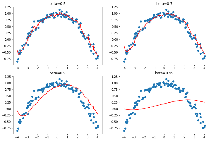
With a large beta, we might miss that the gradients have changed directions and roll over a small local minima. This is a desired side effect: intuitively, when we show a new input to our model, it will look like something in the training set but won’t be exactly like it. That means it will correspond to a point in the loss function that is close to the minimum we ended up with at the end of training, but not exactly at that minimum. So, we would rather end up training in a wide minimum, where nearby points have approximately the same loss (or if you prefer, a point where the loss is as flat as possible). <> shows how the chart in <> varies as we change beta.

In [ ]:

We can see in these examples that a beta that’s too high results in the overall changes in gradient getting ignored. In SGD with momentum, a value of beta that is often used is 0.9.

fit_one_cycle by default starts with a beta of 0.95, gradually adjusts it to 0.85, and then gradually moves it back to 0.95 at the end of training. Let’s see how our training goes with momentum added to plain SGD.

In order to add momentum to our optimizer, we’ll first need to keep track of the moving average gradient, which we can do with another callback. When an optimizer callback returns a , it is used to update the state of the optimizer and is passed back to the optimizer on the next step. So this callback will keep track of the gradient averages in a parameter called grad_avg:

def average_grad(p, mom, grad_avg=None, **kwargs):
    if grad_avg is None: grad_avg = torch.zeros_like(p.grad.data)
    return {'grad_avg': grad_avg*mom + p.grad.data}

To use it, we just have to replace p.grad.data with grad_avg in our step function:

In [ ]:

In [ ]:

opt_func = partial(Optimizer, cbs=[average_grad,momentum_step], mom=0.9)

Learner will automatically schedule mom and lr, so fit_one_cycle will even work with our custom Optimizer:

In [ ]:

In [ ]:

learn.recorder.plot_sched()

We’re still not getting great results, so let’s see what else we can do.