Once you’ve got a model you’re happy with, you need to save it, so that you can then copy it over to a server where you’ll use it in production. Remember that a model consists of two parts: the architecture and the trained parameters. The easiest way to save the model is to save both of these, because that way when you load a model you can be sure that you have the matching architecture and parameters. To save both parts, use the method.

This method even saves the definition of how to create your DataLoaders. This is important, because otherwise you would have to redefine how to transform your data in order to use your model in production. fastai automatically uses your validation set DataLoader for inference by default, so your data augmentation will not be applied, which is generally what you want.

When you call export, fastai will save a file called “export.pkl”:

In [ ]:

Let’s check that the file exists, by using the ls method that fastai adds to Python’s Path class:

In [ ]:

path = Path()
path.ls(file_exts='.pkl')

Out[ ]:

(#1) [Path('export.pkl')]

You’ll need this file wherever you deploy your app to. For now, let’s try to create a simple app within our notebook.

When we use a model for getting predictions, instead of training, we call it inference. To create our inference learner from the exported file, we use load_learner (in this case, this isn’t really necessary, since we already have a working Learner in our notebook; we’re just doing it here so you can see the whole process end-to-end):

In [ ]:

learn_inf = load_learner(path/'export.pkl')

When we’re doing inference, we’re generally just getting predictions for one image at a time. To do this, pass a filename to predict:

In [ ]:

learn_inf.predict('images/grizzly.jpg')

Out[ ]:

('grizzly', tensor(1), tensor([9.0767e-06, 9.9999e-01, 1.5748e-07]))

This has returned three things: the predicted category in the same format you originally provided (in this case that’s a string), the index of the predicted category, and the probabilities of each category. The last two are based on the order of categories in the vocab of the DataLoaders; that is, the stored list of all possible categories. At inference time, you can access the DataLoaders as an attribute of the Learner:

In [ ]:

Out[ ]:

(#3) ['black','grizzly','teddy']

We can see here that if we index into the vocab with the integer returned by predict then we get back “grizzly,” as expected. Also, note that if we index into the list of probabilities, we see a nearly 1.00 probability that this is a grizzly.

We know how to make predictions from our saved model, so we have everything we need to start building our app. We can do it directly in a Jupyter notebook.

To use our model in an application, we can simply treat the predict method as a regular function. Therefore, creating an app from the model can be done using any of the myriad of frameworks and techniques available to application developers.

However, most data scientists are not familiar with the world of web application development. So let’s try using something that you do, at this point, know: it turns out that we can create a complete working web application using nothing but Jupyter notebooks! The two things we need to make this happen are:

• IPython widgets (ipywidgets)
• Voilà

IPython widgets are GUI components that bring together JavaScript and Python functionality in a web browser, and can be created and used within a Jupyter notebook. For instance, the image cleaner that we saw earlier in this chapter is entirely written with IPython widgets. However, we don’t want to require users of our application to run Jupyter themselves.

But we still have the advantage of developing in a notebook, so with ipywidgets, we can build up our GUI step by step. We will use this approach to create a simple image classifier. First, we need a file upload widget:

In [ ]:

#hide_output
btn_upload

Now we can grab the image:

In [ ]:

#hide
# For the book, we can't actually click an upload button, so we fake it

In [ ]:

img = PILImage.create(btn_upload.data[-1])

We can use an Output widget to display it:

In [ ]:

#hide_output
out_pl = widgets.Output()
out_pl.clear_output()
with out_pl: display(img.to_thumb(128,128))
out_pl

Then we can get our predictions:

In [ ]:

and use a Label to display them:

In [ ]:

#hide_output
lbl_pred = widgets.Label()
lbl_pred.value = f'Prediction: {pred}; Probability: {probs[pred_idx]:.04f}'
lbl_pred

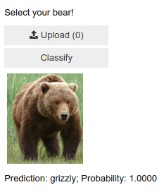
Prediction: grizzly; Probability: 1.0000

We’ll need a button to do the classification. It looks exactly like the upload button:

In [ ]:

#hide_output
btn_run = widgets.Button(description='Classify')
btn_run

We’ll also need a click event handler; that is, a function that will be called when it’s pressed. We can just copy over the lines of code from above:

In [ ]:

def on_click_classify(change):
    out_pl.clear_output()
    with out_pl: display(img.to_thumb(128,128))
    pred,pred_idx,probs = learn_inf.predict(img)
btn_run.on_click(on_click_classify)

You can test the button now by pressing it, and you should see the image and predictions update automatically!

We can now put them all in a vertical box (VBox) to complete our GUI:

#hide
#Putting back btn_upload to a widget for next cell
btn_upload = widgets.FileUpload()

In [ ]:

#hide_output
VBox([widgets.Label('Select your bear!'), 
      btn_upload, btn_run, out_pl, lbl_pred])

We have written all the code necessary for our app. The next step is to convert it into something we can deploy.

In [ ]:

Now that we have everything working in this Jupyter notebook, we can create our application. To do this, start a new notebook and add to it only the code needed to create and show the widgets that you need, and markdown for any text that you want to appear. Have a look at the bear_classifier notebook in the book’s repo to see the simple notebook application we created.

Next, install Voilà if you haven’t already, by copying these lines into a notebook cell and executing it:

!pip install voila
!jupyter serverextension enable --sys-prefix voila

Cells that begin with a ! do not contain Python code, but instead contain code that is passed to your shell (bash, Windows PowerShell, etc.). If you are comfortable using the command line, which we’ll discuss more later in this book, you can of course simply type these two lines (without the ! prefix) directly into your terminal. In this case, the first line installs the voila library and application, and the second connects it to your existing Jupyter notebook.

Voilà runs Jupyter notebooks just like the Jupyter notebook server you are using now does, but it also does something very important: it removes all of the cell inputs, and only shows output (including ipywidgets), along with your markdown cells. So what’s left is a web application! To view your notebook as a Voilà web application, replace the word “notebooks” in your browser’s URL with: “voila/render”. You will see the same content as your notebook, but without any of the code cells.

Of course, you don’t need to use Voilà or ipywidgets. Your model is just a function you can call (pred,pred_idx,probs = learn.predict(img)), so you can use it with any framework, hosted on any platform. And you can take something you’ve prototyped in ipywidgets and Voilà and later convert it into a regular web application. We’re showing you this approach in the book because we think it’s a great way for data scientists and other folks that aren’t web development experts to create applications from their models.

We have our app, now let’s deploy it!

As you now know, you need a GPU to train nearly any useful deep learning model. So, do you need a GPU to use that model in production? No! You almost certainly do not need a GPU to serve your model in production. There are a few reasons for this:

• As we’ve seen, GPUs are only useful when they do lots of identical work in parallel. If you’re doing (say) image classification, then you’ll normally be classifying just one user’s image at a time, and there isn’t normally enough work to do in a single image to keep a GPU busy for long enough for it to be very efficient. So, a CPU will often be more cost-effective.
• An alternative could be to wait for a few users to submit their images, and then batch them up and process them all at once on a GPU. But then you’re asking your users to wait, rather than getting answers straight away! And you need a high-volume site for this to be workable. If you do need this functionality, you can use a tool such as Microsoft’s , or AWS Sagemaker
• The complexities of dealing with GPU inference are significant. In particular, the GPU’s memory will need careful manual management, and you’ll need a careful queueing system to ensure you only process one batch at a time.
• There’s a lot more market competition in CPU than GPU servers, as a result of which there are much cheaper options available for CPU servers.

Because of the complexity of GPU serving, many systems have sprung up to try to automate this. However, managing and running these systems is also complex, and generally requires compiling your model into a different form that’s specialized for that system. It’s typically preferable to avoid dealing with this complexity until/unless your app gets popular enough that it makes clear financial sense for you to do so.

For at least the initial prototype of your application, and for any hobby projects that you want to show off, you can easily host them for free. The best place and the best way to do this will vary over time, so check the for the most up-to-date recommendations. As we’re writing this book in early 2020 the simplest (and free!) approach is to use Binder. To publish your web app on Binder, you follow these steps:

1. Add your notebook to a .
2. Paste the URL of that repo into Binder’s URL, as shown in <>.
3. Change the File dropdown to instead select URL.
4. In the “URL to open” field, enter /voila/render/name.ipynb (replacing name with the name of for your notebook).
5. Click Launch.

The first time you do this, Binder will take around 5 minutes to build your site. Behind the scenes, it is finding a virtual machine that can run your app, allocating storage, collecting the files needed for Jupyter, for your notebook, and for presenting your notebook as a web application.

Finally, once it has started the app running, it will navigate your browser to your new web app. You can share the URL you copied to allow others to access your app as well.

For other (both free and paid) options for deploying your web app, be sure to take a look at the book’s website.

You may well want to deploy your application onto mobile devices, or edge devices such as a Raspberry Pi. There are a lot of libraries and frameworks that allow you to integrate a model directly into a mobile application. However, these approaches tend to require a lot of extra steps and boilerplate, and do not always support all the PyTorch and fastai layers that your model might use. In addition, the work you do will depend on what kind of mobile devices you are targeting for deployment—you might need to do some work to run on iOS devices, different work to run on newer Android devices, different work for older Android devices, etc. Instead, we recommend wherever possible that you deploy the model itself to a server, and have your mobile or edge application connect to it as a web service.

There are quite a few upsides to this approach. The initial installation is easier, because you only have to deploy a small GUI application, which connects to the server to do all the heavy lifting. More importantly perhaps, upgrades of that core logic can happen on your server, rather than needing to be distributed to all of your users. Your server will have a lot more memory and processing capacity than most edge devices, and it is far easier to scale those resources if your model becomes more demanding. The hardware that you will have on a server is also going to be more standard and more easily supported by fastai and PyTorch, so you don’t have to compile your model into a different form.

There are downsides too, of course. Your application will require a network connection, and there will be some latency each time the model is called. (It takes a while for a neural network model to run anyway, so this additional network latency may not make a big difference to your users in practice. In fact, since you can use better hardware on the server, the overall latency may even be less than if it were running locally!) Also, if your application uses sensitive data then your users may be concerned about an approach which sends that data to a remote server, so sometimes privacy considerations will mean that you need to run the model on the edge device (it may be possible to avoid this by having an on-premise server, such as inside a company’s firewall). Managing the complexity and scaling the server can create additional overhead too, whereas if your model runs on the edge devices then each user is bringing their own compute resources, which leads to easier scaling with an increasing number of users (also known as horizontal scaling).

Congratulations, you have successfully built a deep learning model and deployed it! Now is a good time to take a pause and think about what could go wrong.