
- It works even when our dependent variable has more than two categories.
- It results in faster and more reliable training.
In order to understand how cross-entropy loss works for dependent variables with more than two categories, we first have to understand what the actual data and activations that are seen by the loss function look like.
Let’s take a look at the activations of our model. To actually get a batch of real data from our , we can use the one_batch method:
In [ ]:
As you see, this returns the dependent and independent variables, as a mini-batch. Let’s see what is actually contained in our dependent variable:
In [ ]:
y
Out[ ]:
TensorCategory([ 0, 5, 23, 36, 5, 20, 29, 34, 33, 32, 31, 24, 12, 36, 8, 26, 30, 2, 12, 17, 7, 23, 12, 29, 21, 4, 35, 33, 0, 20, 26, 30, 3, 6, 36, 2, 17, 32, 11, 6, 3, 30, 5, 26, 26, 29, 7, 36,31, 26, 26, 8, 13, 30, 11, 12, 36, 31, 34, 20, 15, 8, 8, 23], device='cuda:5')
Our batch size is 64, so we have 64 rows in this tensor. Each row is a single integer between 0 and 36, representing our 37 possible pet breeds. We can view the predictions (that is, the activations of the final layer of our neural network) using Learner.get_preds. This function either takes a dataset index (0 for train and 1 for valid) or an iterator of batches. Thus, we can pass it a simple list with our batch to get our predictions. It returns predictions and targets by default, but since we already have the targets, we can effectively ignore them by assigning to the special variable _:
In [ ]:
preds,_ = learn.get_preds(dl=[(x,y)])preds[0]
Out[ ]:
tensor([9.9911e-01, 5.0433e-05, 3.7515e-07, 8.8590e-07, 8.1794e-05, 1.8991e-05, 9.9280e-06, 5.4656e-07, 6.7920e-06, 2.3486e-04, 3.7872e-04, 2.0796e-05, 4.0443e-07, 1.6933e-07, 2.0502e-07, 3.1354e-08,9.4115e-08, 2.9782e-06, 2.0243e-07, 8.5262e-08, 1.0900e-07, 1.0175e-07, 4.4780e-09, 1.4285e-07, 1.0718e-07, 8.1411e-07, 3.6618e-07, 4.0950e-07, 3.8525e-08, 2.3660e-07, 5.3747e-08, 2.5448e-07,6.5860e-08, 8.0937e-05, 2.7464e-07, 5.6760e-07, 1.5462e-08])
The actual predictions are 37 probabilities between 0 and 1, which add up to 1 in total:
In [ ]:
len(preds[0]),preds[0].sum()
Out[ ]:
(37, tensor(1.0000))
To transform the activations of our model into predictions like this, we used something called the softmax activation function.
In our classification model, we use the softmax activation function in the final layer to ensure that the activations are all between 0 and 1, and that they sum to 1.
Softmax is similar to the sigmoid function, which we saw earlier. As a reminder sigmoid looks like this:
In [ ]:
plot_function(torch.sigmoid, min=-4,max=4)
We can apply this function to a single column of activations from a neural network, and get back a column of numbers between 0 and 1, so it’s a very useful activation function for our final layer.
Now think about what happens if we want to have more categories in our target (such as our 37 pet breeds). That means we’ll need more activations than just a single column: we need an activation per category. We can create, for instance, a neural net that predicts 3s and 7s that returns two activations, one for each class—this will be a good first step toward creating the more general approach. Let’s just use some random numbers with a standard deviation of 2 (so we multiply randn by 2) for this example, assuming we have 6 images and 2 possible categories (where the first column represents 3s and the second is 7s):
In [ ]:
#hidetorch.random.manual_seed(42);
In [ ]:
acts = torch.randn((6,2))*2acts
Out[ ]:
tensor([[ 0.6734, 0.2576],[ 0.4689, 0.4607],[-2.2457, -0.3727],[ 4.4164, -1.2760],[ 0.9233, 0.5347],[ 1.0698, 1.6187]])
We can’t just take the sigmoid of this directly, since we don’t get rows that add to 1 (i.e., we want the probability of being a 3 plus the probability of being a 7 to add up to 1):
In [ ]:
Out[ ]:
tensor([[0.6623, 0.5641],[0.6151, 0.6132],[0.0957, 0.4079],[0.9881, 0.2182],[0.7157, 0.6306],[0.7446, 0.8346]])
In <>, our neural net created a single activation per image, which we passed through the sigmoid function. That single activation represented the model’s confidence that the input was a 3. Binary problems are a special case of classification problems, because the target can be treated as a single boolean value, as we did in mnist_loss. But binary problems can also be thought of in the context of the more general group of classifiers with any number of categories: in this case, we happen to have two categories. As we saw in the bear classifier, our neural net will return one activation per category.
So in the binary case, what do those activations really indicate? A single pair of activations simply indicates the relative confidence of the input being a 3 versus being a 7. The overall values, whether they are both high, or both low, don’t matter—all that matters is which is higher, and by how much.
We would expect that since this is just another way of representing the same problem, that we would be able to use sigmoid directly on the two-activation version of our neural net. And indeed we can! We can just take the difference between the neural net activations, because that reflects how much more sure we are of the input being a 3 than a 7, and then take the sigmoid of that:
Out[ ]:
tensor([0.6025, 0.5021, 0.1332, 0.9966, 0.5959, 0.3661])
The second column (the probability of it being a 7) will then just be that value subtracted from 1. Now, we need a way to do all this that also works for more than two columns. It turns out that this function, called softmax, is exactly that:
def softmax(x): return exp(x) / exp(x).sum(dim=1, keepdim=True)
Let’s check that softmax returns the same values as sigmoid for the first column, and those values subtracted from 1 for the second column:
In [ ]:
sm_acts
Out[ ]:
tensor([[0.6025, 0.3975],[0.5021, 0.4979],[0.1332, 0.8668],[0.9966, 0.0034],[0.5959, 0.4041],[0.3661, 0.6339]])
softmax is the multi-category equivalent of sigmoid—we have to use it any time we have more than two categories and the probabilities of the categories must add to 1, and we often use it even when there are just two categories, just to make things a bit more consistent. We could create other functions that have the properties that all activations are between 0 and 1, and sum to 1; however, no other function has the same relationship to the sigmoid function, which we’ve seen is smooth and symmetric. Also, we’ll see shortly that the softmax function works well hand-in-hand with the loss function we will look at in the next section.
If we have three output activations, such as in our bear classifier, calculating softmax for a single bear image would then look like something like <>.
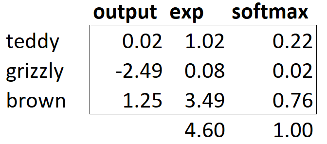
What does this function do in practice? Taking the exponential ensures all our numbers are positive, and then dividing by the sum ensures we are going to have a bunch of numbers that add up to 1. The exponential also has a nice property: if one of the numbers in our activations x is slightly bigger than the others, the exponential will amplify this (since it grows, well… exponentially), which means that in the softmax, that number will be closer to 1.
Intuitively, the softmax function really wants to pick one class among the others, so it’s ideal for training a classifier when we know each picture has a definite label. (Note that it may be less ideal during inference, as you might want your model to sometimes tell you it doesn’t recognize any of the classes that it has seen during training, and not pick a class because it has a slightly bigger activation score. In this case, it might be better to train a model using multiple binary output columns, each using a sigmoid activation.)
Softmax is the first part of the cross-entropy loss—the second part is log likelihood.
When we calculated the loss for our MNIST example in the last chapter we used:
def mnist_loss(inputs, targets):inputs = inputs.sigmoid()return torch.where(targets==1, 1-inputs, inputs).mean()
Just as we moved from sigmoid to softmax, we need to extend the loss function to work with more than just binary classification—it needs to be able to classify any number of categories (in this case, we have 37 categories). Our activations, after softmax, are between 0 and 1, and sum to 1 for each row in the batch of predictions. Our targets are integers between 0 and 36.
In the binary case, we used torch.where to select between inputs and 1-inputs. When we treat a binary classification as a general classification problem with two categories, it actually becomes even easier, because (as we saw in the previous section) we now have two columns, containing the equivalent of inputs and 1-inputs. So, all we need to do is select from the appropriate column. Let’s try to implement this in PyTorch. For our synthetic 3s and 7s example, let’s say these are our labels:
In [ ]:
targ = tensor([0,1,0,1,1,0])
and these are the softmax activations:
In [ ]:
sm_acts
Out[ ]:
tensor([[0.6025, 0.3975],[0.5021, 0.4979],[0.1332, 0.8668],[0.9966, 0.0034],[0.5959, 0.4041],[0.3661, 0.6339]])
Then for each item of targ we can use that to select the appropriate column of sm_acts using tensor indexing, like so:
In [ ]:
sm_acts[idx, targ]
Out[ ]:
tensor([0.6025, 0.4979, 0.1332, 0.0034, 0.4041, 0.3661])
To see exactly what’s happening here, let’s put all the columns together in a table. Here, the first two columns are our activations, then we have the targets, the row index, and finally the result shown immediately above:
In [ ]:
#hide_inputfrom IPython.display import HTMLdf = pd.DataFrame(sm_acts, columns=["3","7"])df['targ'] = targdf['idx'] = idxdf['loss'] = sm_acts[range(6), targ]t = df.style.hide_index()#To have html code compatible with our scripthtml = t._repr_html_().split('</style>')[1]html = re.sub(r'<table id="([^"]+)"\s*>', r'<table >', html)display(HTML(html))
Looking at this table, you can see that the final column can be calculated by taking the targ and columns as indices into the two-column matrix containing the 3 and 7 columns. That’s what sm_acts[idx, targ] is actually doing.
The really interesting thing here is that this actually works just as well with more than two columns. To see this, consider what would happen if we added an activation column for every digit (0 through 9), and then targ contained a number from 0 to 9. As long as the activation columns sum to 1 (as they will, if we use softmax), then we’ll have a loss function that shows how well we’re predicting each digit.
We’re only picking the loss from the column containing the correct label. We don’t need to consider the other columns, because by the definition of softmax, they add up to 1 minus the activation corresponding to the correct label. Therefore, making the activation for the correct label as high as possible must mean we’re also decreasing the activations of the remaining columns.
PyTorch provides a function that does exactly the same thing as sm_acts[range(n), targ] (except it takes the negative, because when applying the log afterward, we will have negative numbers), called nll_loss (NLL stands for negative log likelihood):
-sm_acts[idx, targ]
Out[ ]:
In [ ]:
F.nll_loss(sm_acts, targ, reduction='none')
Out[ ]:
tensor([-0.6025, -0.4979, -0.1332, -0.0034, -0.4041, -0.3661])
Despite its name, this PyTorch function does not take the log. We’ll see why in the next section, but first, let’s see why taking the logarithm can be useful.
The function we saw in the previous section works quite well as a loss function, but we can make it a bit better. The problem is that we are using probabilities, and probabilities cannot be smaller than 0 or greater than 1. That means that our model will not care whether it predicts 0.99 or 0.999. Indeed, those numbers are so close together—but in another sense, 0.999 is 10 times more confident than 0.99. So, we want to transform our numbers between 0 and 1 to instead be between negative infinity and 0. There is a mathematical function that does exactly this: the logarithm (available as torch.log). It is not defined for numbers less than 0, and looks like this:
In [ ]:
plot_function(torch.log, min=0,max=4)
Does “logarithm” ring a bell? The logarithm function has this identity:
y = b**aa = log(y,b)
In this case, we’re assuming that log(y,b) returns log y base b. However, PyTorch actually doesn’t define log this way: log in Python uses the special number e (2.718…) as the base.
Perhaps a logarithm is something that you have not thought about for the last 20 years or so. But it’s a mathematical idea that is going to be really critical for many things in deep learning, so now would be a great time to refresh your memory. The key thing to know about logarithms is this relationship:
log(a*b) = log(a)+log(b)
When we see it in that format, it looks a bit boring; but think about what this really means. It means that logarithms increase linearly when the underlying signal increases exponentially or multiplicatively. This is used, for instance, in the Richter scale of earthquake severity, and the dB scale of noise levels. It’s also often used on financial charts, where we want to show compound growth rates more clearly. Computer scientists love using logarithms, because it means that multiplication, which can create really really large and really really small numbers, can be replaced by addition, which is much less likely to result in scales that are difficult for our computers to handle.
Taking the mean of the positive or negative log of our probabilities (depending on whether it’s the correct or incorrect class) gives us the negative log likelihood loss. In PyTorch, nll_loss assumes that you already took the log of the softmax, so it doesn’t actually do the logarithm for you.
When we first take the softmax, and then the log likelihood of that, that combination is called cross-entropy loss. In PyTorch, this is available as nn.CrossEntropyLoss (which, in practice, actually does log_softmax and then nll_loss):
In [ ]:
loss_func = nn.CrossEntropyLoss()
As you see, this is a class. Instantiating it gives you an object which behaves like a function:
In [ ]:
loss_func(acts, targ)
Out[ ]:
tensor(1.8045)
All PyTorch loss functions are provided in two forms, the class just shown above, and also a plain functional form, available in the F namespace:
In [ ]:
F.cross_entropy(acts, targ)
Out[ ]:
tensor(1.8045)
Either one works fine and can be used in any situation. We’ve noticed that most people tend to use the class version, and that’s more often used in PyTorch’s official docs and examples, so we’ll tend to use that too.
By default PyTorch loss functions take the mean of the loss of all items. You can use reduction='none' to disable that:
In [ ]:
nn.CrossEntropyLoss(reduction='none')(acts, targ)
Out[ ]:
tensor([0.5067, 0.6973, 2.0160, 5.6958, 0.9062, 1.0048])
We have now seen all the pieces hidden behind our loss function. But while this puts a number on how well (or badly) our model is doing, it does nothing to help us know if it’s actually any good. Let’s now see some ways to interpret our model’s predictions.

